A while ago I sat in a meeting and had one of the people I work with explain to me, why re-sampling before doing classification* was “the way to go in that kind of situation”. After trying to point out a few risks with that approach I was only met with an “I don’t believe that. Prove that to me.” – answer.
* As pointed out by u/nico_25 in r/MachineLearning my choice of wording was really bad here. Please read here: “hypothesis testing in regards to treatment effectiveness”. The team I worked in during that time always used the term “classification” to describe “let’s classify whether or not that treatment is effective”. Even though I was trying to paint a picture, adopting that formulation is not okay.
Since a theoretical proof/discussion is sometimes not the right way to go, I constructed a little example showcasing what could happen. After that I’ve ran into the same kind of situation for a few times, so I decided to write it down, hoping it could help some people.
So what exactly was “that kind of situation”?
The initial situation
Lets assume we got a trial to perform (a quiz, a medical treatment, a questionnaire, …) with 1000 people. We know four things about them:
- Age (from 18 to 85)
- Highest Education (High School, College, University)
- Gender (Male, Female)
The fourth information is whether they passed the trial successfully or not. Unfortunately of all these people only about 30 are in the class success. That means 97% of all rows in our dataset have got an unsuccessful outcome. Most (simple) classifiers won’t get the best results, simply because our classes are extremely imbalanced.
On a side note: One of the many problems with imbalanced classes is the way we try to evaluate the chosen classifier. Accuracy, although easily understood as a measurement, can often be quite misleading. A deeper look into that topic would be too much for this post, but this CrossValidated thread serves as a good entry point.
In the following paragraphs we’ll construct an artificial dataset and investigate what actually happens as soon as we apply a simple re-sampling algorithm to it. I’ll provide a few snippets of the R code/output (you won’t need any prior R knowledge to follow!) that I used. You can find the complete code at the bottom of the page.
Generating the data
As stated above, we assume a population of 1000 people with three stats and an outcome each. We’ll chose age, education and gender randomly. The outcome only depends on age; education and gender only represent some kind of noise.
n <- 1000

age <- sample(18:85, size=n, replace=TRUE)
edu <- sample(c("high school", "college", "university"), size=n, replace=TRUE)
sex <- sample(c("male", "female"), size=n, replace=T)

res <- runif(n)*0.95 + age/85*0.05 > 0.95
As you can see the trial-outcome (res) is a weighted combination of a random number (uniformly distributed between 0 and 1) and the age of the patient (with age having a small but positive effect). We will end up with the following data:
     age            sex            edu             res
Min.   :18.00   female:515   college    :350   FALSE:972
Mean   :51.99   male  :485   high school:344   TRUE :28
Max.   :85.00                university :306
This shows pretty much evenly distributed values for gender and education as well as 28 successful outcomes out of 1000 tries. For ease of understanding the results, we’ll perform our analysis using a simple logistic regression (you can of course use other methods like RandomForests, Classification Trees, … and observe a similar effect).
Analysis of the original data
Looking at a simple model (made with glm) we can already see a small positive effect of age on our outcome:
Coefficients:
               Estimate Std. Error z value Pr(>|z|)
(Intercept)    -4.88685    0.71676  -6.818 9.23e-12 ***
age             0.02211    0.01022   2.163   0.0305 *
sexmale         0.06268    0.38466   0.163   0.8706
eduhigh school  0.11152    0.46708   0.239   0.8113
eduuniversity   0.09909    0.47982   0.207   0.8364
Here the column “Estimate” gives us the estimated coefficient while “Pr(>|z|)” displays the corresponding p-value (in a nutshell: smaller means we are more sure that variable really has an effect on our outcome).
Therefore we can observe that gender and education show no significant effect. But why is that even important, since we already know, that we constructed these two values to only act as random noise? Think about it that way: We don’t know what our random construction did – depending on seed it could (theoretically) happen, that every successful outcome has gender “female” and vice versa. Then – even though not planned for – there would actually be a measurable effect of gender.
To clarify a bit on the given output: Like with education, just the estimator male is shown for our input gender. That’s due to the fact, that all these multi-factor variables are being “normalized” on one of their factor-values, which influences the estimated value of our intercept. Therefore a positive value for male would indicate, that men are more likely to succeed than women (which isn’t the case here with a p-value of 0.87).
Re-sampling
There are two super-easy methods to better balance our classes:
- Under-sampling and
- Over-sampling
Under-sampling simply discards some of the rows of our dominant class until we reach a given ratio. If we aim for a 1:1 ratio between success and no success that would leave us with 56 samples. Since that is not enough (and we would’ve just discarded 94% of our dataset) we’ll try a basic over-sampling method: Pick random rows that describe a success until we got enough “new” data that, when combining it with our original data, our classes are balanced.
Take a look at this image from svds.com to better understand the difference of these methods:
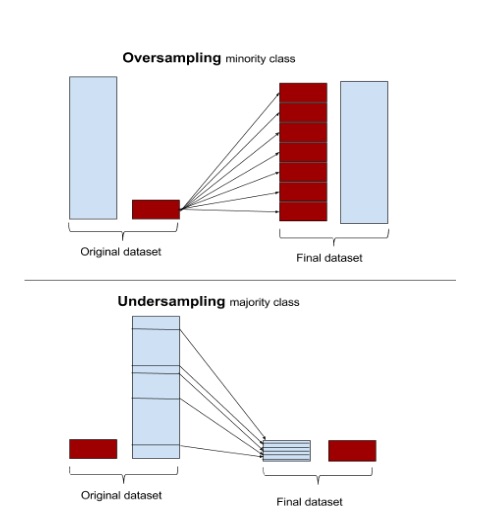
It may seem like over-sampling would be far superior. After all we aren’t loosing any data and even end up with more than we started. But be careful: there isn’t any new data being generated, it’s all just copies of existing entries. Therefore we aren’t gaining any new insights and we are in some way amplifying our noise.
Analysis of our artificial data
Now that we’ve got balanced classes we once again use a logistic regression and take a look at its results:
Coefficients:
                 Estimate Std. Error z value Pr(>|z|)
(Intercept)    -1.617702   0.175712  -9.207  < 2e-16 ***
age             0.025623   0.002620   9.781  < 2e-16 ***
sexmale         0.008431   0.094359   0.089  0.92880
eduhigh school  0.212338   0.114104   1.861  0.06276 .
eduuniversity   0.329840   0.116985   2.820  0.00481 **
First of all we notice an increased significance of the variable age. You can also see that the estimated coefficient has changed. We already induced a small deviation compared to our original data. But wait - there's more!!
Suddenly our model tells us, that completing a university could greatly benefit our chance to be successful (compared to college). Where does that information come from and can it even be correct? To answer that, we'll take a look at our original dataset.
| education/outcome | no success | success |
| high school | 334 | 10 |
| college | 341 | 9 |
| university | 297 | 9 |
As you can see the education level is nearly balanced (350, 344, 306). Also - when comparing persons that went to college / university - we can see, that there are exactly nine patients each that had a successful outcome.
During our over-sampling process we randomly draw from these 28 successful people. We would therefore assume, that the distribution of people (regarding their education) in our artificial dataset would be the same. Now lets take a look at how our over-sampled data looks like:
| education/outcome | no success | success |
| high school | 334 | 340 |
| college | 341 | 300 |
| university | 297 | 332 |
Suddenly there are 10% more people that went to university and were successful - compared to what we would expect when looking at the college row. This makes it look like going to university actually helps - when in reality it has no influence.
But why does this happen?
The answer is simple. Since we are drawing random people out of the "successful"-bag we will get duplicates. Because random does really mean random after all (and not perfectly balanced), there will always be people who get picked more often than others. If this happens to favor people from university, we'll end up with a higher success-rate for them.
Whether or not a variable has some effect on outcome in our original dataset can't easily be said with only looking at the output of our over-sampled data. Certainly we can't for sure conclude from a "nice" result after over-sampling that this exact finding holds true when applying it to our original data.
How to avoid these problems?
There are a multitude of approaches out there to handle imbalanced classes. Especially in the field of re-sampling there are many different methods - with the showcased "random naive over-sampling" being one of the most basic ones.
If you are interested in more specific approaches, ADASYN or SMOTE could be decent starting points when using R. Although scikit-learn isn't an R package and has been criticized a few times (recent discussion) it's used by a lot of people and provides some really good docs.
Therefore I'll recommend taking a look at the imbalanced-learn repository or read/work through some examples on their page. This provides you with a rather extensive list of algorithms that you can further explore. If you'd like to stick to Python and are looking for an easy introduction, here is a quick read on SMOTE and ADASYN with imblearn.
Final words
I won't - for now - go further into more complex ways to re-sample your data. If there are more people interested in stuff like that, I'll maybe do a follow-up. As promised you can find the whole code that was used to generate this short example here.
Re-sampling per se isn't bad and is often times the right approach to your problem. One just has to be careful of the consequences and not blindly throw algorithms at some data without a basic understanding of what actually goes on. The most important thought (in my opinion) to take away is:
Always think about how every step changes your data and what kind of impact that could potentially have on your results.